Imagine the following situation. You are testing the linearity of an analytical method, let’s say HPLC. The linearity coefficient is R=0.999, the coefficient of determination is R2 = 0.999. An ideal situation. The criteria are met, the validation is successful. Now all that’s left is to write the report and go home. Nothing could be further from the truth. There may be a hidden gremlin in our data that is not visible at first glance. However, residual analysis will help us with this.

Linearity and regression model fit
In 2023, the ICH published a new guideline, ICH Q2 – Validation of Analytical Methods. One of the changes concerned the determination of linearity. The new guidelines took into account biological methods such as ELISA and cytotoxicity tests. These methods are often based on non-linear calibration models. Therefore, it is impossible to determine their linearity.
For this reason, linearity has been replaced by regression model fitting in the new ICH Q2. This does not change the fact that the term linearity can still be used for methods that are linear in nature.
How does linear regression work?
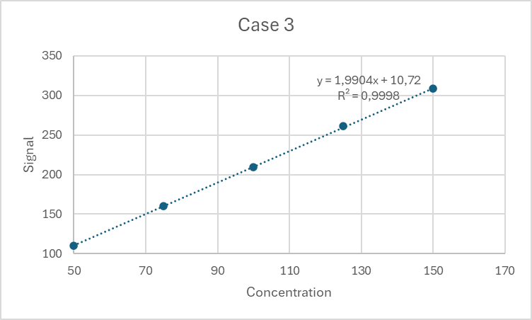
In order to determine the concentration, a calibration curve is constructed. Several solutions of known concentration are analysed and, based on the results obtained, a graph of the linear dependence of the signal on the concentration is generated. Of course, the measured values may not coincide perfectly with the curve. Therefore, interpolation is used, in which the line of the graph runs between the measured points. The course is not random and is determined so that the sum of the squares of the measurement errors is the smallest.
Linearity coefficient and coefficient of determination
When determining linearity and reading results, we may encounter two values: the linearity coefficient – R, and the coefficient of determination – R2. How do they differ?
Linearity coefficient (R) – identical to Pearson’s correlation coefficient. It indicates whether the relationship between data is linear and to what extent. The closer the value is to 1, the stronger the correlation.
Coefficient of determination (R²) – This is calculated by squaring the R value. It indicates the fit of the regression model, i.e. how well the concentration can be determined based on the signal measurement.
OK, our data is perfect: linearity coefficient R = 0.9999, coefficient of determination R2 = 0.9999? Well, theoretically, the model is a perfect fit. Perhaps even accuracy would not reveal any problems. However, it is possible that we are calculating something wrong and our method is even more accurate than we think.
Residual analysis – is the model truly linear?
Residual analysis is one of the stages of regression model evaluation. It involves examining the differences (residuals) between the observed (measured) values and the values read from the regression model. The residuals (e) represent model errors. Their position on the concentration dependence graph can indicate whether the model is properly fitted.

Analysis of the graph showing the relationship between concentration and residual values can help to determine the following:
- Verification of model correctness
- Verification of variance homogeneity (homoscedasticity)
- Identification of outliers
To explain residual analysis, we will use the following data set:
| Concentration | Signal |
| 50 | 110,2483571 |
| 75 | 159,9308678 |
| 100 | 210,3238443 |
| 125 | 260,7615149 |
| 150 | 309,8829233 |
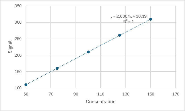
The signal represents the measured values. To calculate the residuals, we need to determine the expected values based on the equation of the curve y=ax +b.
| Concentration | Signal (y) | Expected values (ŷ) |
| 50 | 110,2483571 | 110,2095456 |
| 75 | 159,9308678 | 160,2195235 |
| 100 | 210,3238443 | 210,2295015 |
| 125 | 260,7615149 | 260,2394794 |
| 150 | 309,8829233 | 310,2494574 |
Then, using the difference between the measured values and the expected values, we determine the remainders.
| Concentration | Signal (y) | Expected values (ŷ) | Residuals (e) |
| 50 | 110,2483571 | 110,2095456 | 0,038811 |
| 75 | 159,9308678 | 160,2195235 | -0,28866 |
| 100 | 210,3238443 | 210,2295015 | 0,094343 |
| 125 | 260,7615149 | 260,2394794 | 0,522035 |
| 150 | 309,8829233 | 310,2494574 | -0,36653 |
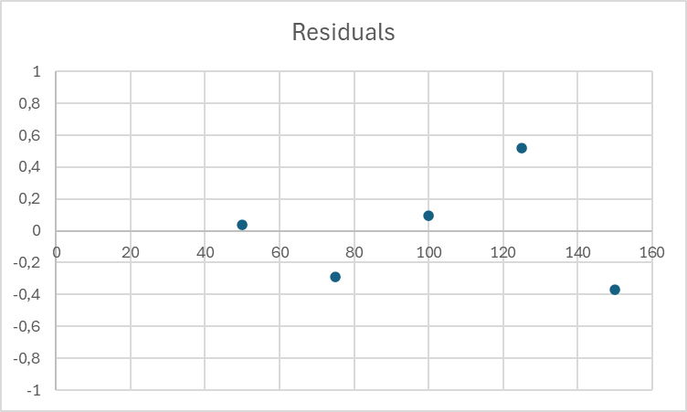
In general:
- The residual values should be evenly distributed on both sides of the horizontal line 0.
- No clear trend or shape indicates a good fit for the linear model.
- Outliers can be observed.
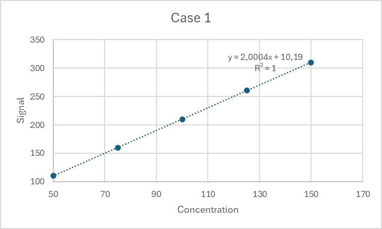
Case study
To demonstrate the true power of residual analysis, I will use a set of three data points.
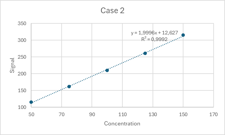
| Case 1 | Case 2 | Case 3 | ||||
| Cocncentration | Signal | Residuals | Signal | Residuals | Signal | Residuals |
| 50 | 110,2483571 | 0,0388115 | 114,9531726 | 2,345937031 | 109,80000 | -0,440000 |
| 75 | 159,9308678 | -0,288655683 | 161,5658426 | -1,031487151 | 160,40000 | 0,400000 |
| 100 | 210,3238443 | 0,094342782 | 210,1534869 | -2,433936904 | 209,20000 | -0,560000 |
| 125 | 260,7615149 | 0,522035486 | 261,1561051 | -1,421412863 | 261,20000 | 1,680000 |
| 150 | 309,8829233 | -0,366534085 | 315,108512 | 2,540899887 | 308,20000 | -1,080000 |
The residual plots for these cases are as follows:
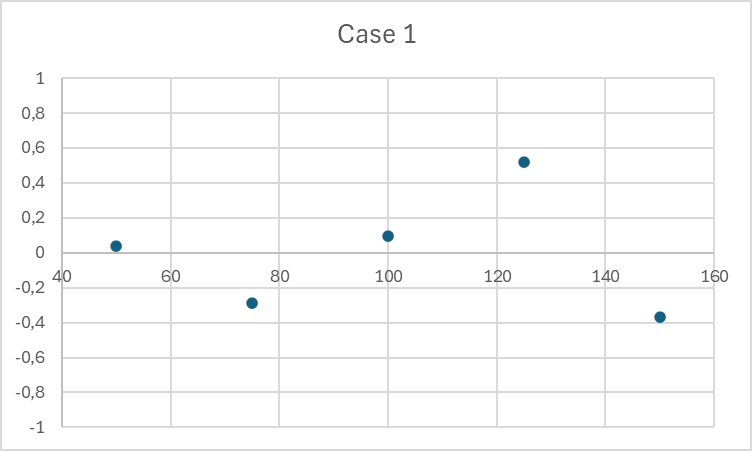
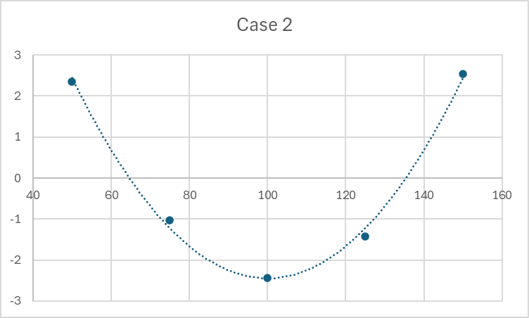
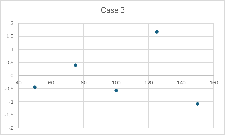
What can we conclude from the graphs?
Case 1:
The points are evenly distributed on both sides of the value 0. There is no clear trend in the position of the points. This indicates a good fit for the linear model.
Case 2:
The characteristic parabolic shape of the points. This shape indicates the non-linear nature of the distribution of points. In most cases, they have a binomial distribution (second-degree function). In this case, the use of a linear model is incorrect despite the high R2 value, as the relationship is non-linear.
Case 3:
The residuals move away from 0 as the concentration increases (funnel shape). This indicates heteroscedasticity. In this case, weighted regression should be used.
Summary
Based on the above data, it is quite clear that the values of R or R2 can be misleading. When determining linearity, it is worth taking a closer look at the data and assessing whether the calibration model we have used is actually the best and consistent with mathematics.
Unfortunately, in most cases, the software used to operate the equipment and analyse the results will not perform this analysis. It is therefore worth using special statistical tools such as Statistica or Minitab, or simply a spreadsheet, to assess whether the linearity is actually linear.